1. Introduction

During the late 2000s, the water level of Lake Enriquillo rose dramatically, and its effects have been reported by massive media including BBC, ABC, The New York Times and local papers. This, in the form of a significant loss of agricultural land, has affected thousands of nearby residents (ARCHIBOLD 2014, Arroyo 2014, Bobylev 2009, Dominican-Today 2013). The causes of the rise, still being debated, might be a combination of increased, above-annual-average rainfall in recent years, increased lake sedimentation and a concomitant lakebed rise due to deforestation-induced run-off, and a reduced surface evaporation rate resulting from milder temperatures (Ramirez 2012). Other causes, such as blocking of the San Cristobal drainage channel located to the southeast of the lake, changes to the lake-floor permeability or lake-floor rise due to seismic activity along the Enriquillo and Los Muertos through fault lines, also have been suggested. In order to explain the water area change of Lake Enriquillo during the 2001-2012 period, some hypotheses have been formulated: 1) land cover and land use changes; 2) hydro-climate change; 3) moisture increment due to increased Sea Surface Temperature (SST) surrounding the lake basin; 4) lake bed sedimentation; 5) seismic activity, and 6) underground water flow change or seawater encroachment into the Lake Enriquillo. We herein will reexamine these hypotheses based on the outcomes of the present study.

There are numerous researches using several types of remote sensing techniques to analyze and manage water area of large lake. Hope et al. (1999) were successful when using linear mixture model to extract the North Slope lake area with the Advanced Very High Resolution Radiometer (AVHRR) data, coarse optical satellite images. The spatial limitation of AVHRR was compensated with lake fraction map. The spatial limitation of coarse image might be treated by combining with higher resolution one (Michishita et al. 2012a). In the research, Poyang Lake area and Great Salt area were mapped by using bi-sensor Landsat TM and Terra Moderate Resolution Imaging Spectroradiometer (MODIS) data and Multiple Endmember Spectral Mixture Analysis (MESMA) technique; however, for this point, data acquisition is another restriction. Regarding water area variation monitoring, MODIS and Landsat are also most widely used with various image classification algorithms. Lakes in the middle Yangtze region were digitized manually on Landsat and available maps over 20^th century, then decreased lake areas was caused by human activities and natural processes (Du et al. 2011). Poyang Lake water body was created annually temporally by Landsat with the Normalized Difference Water Index (NDWI) and the Modified Normalized Difference Water Index (MNDWI) in order to analyze seasonal changing and water inundation (Hui et al. 2008). It is found that MNDWI accuracy is better than NDWI and insufficient to provide accurate estimation of the spatial-temporal process of water inundation over the marshlands through linear interpolation. Three supervised image classification methods (density slicing, classification trees, and feature extraction) were examined based on Landsat TM and ETM+ (Roach et al. 2012). It indicated that the simplest method, density slicing performed best overall. Change in area of Ebinur Lake, China was figured out by using Spot/vegetation image with Normalized Difference Vegetation Index (NDVI) and NDWI (MA et al. 2007). They achieved accuracy at 91.4 when multi-spectral vegetation data is applicable. Water surface variation in Donting lake area, China was monitored successfully by using long-term Terra/ MODIS data time series (Huang et al. 2012). In the research, an integrated threshold of NDWI and NDVI is adopted along with SRTM (Shuttle Radar Topography Mission); then the result was used to analyze flood hazard.

The objectives of this study were to extract water area in a 2001-2012 time-series for mapping and assessment of the spatial patterns of the water area changes of Lake Enriquillo in the Dominican Republic. This saline, terminal lake, the largest and most important in the Dominican Republic, is located on the central plateau of Hispaniola, along with the border with Haiti. Recently the lake has undergone unusual water area changes, the causes of which are as yet unexplained. This paper introduces a MESMA method that utilizes sub-pixel MODIS images to produce water-cover maps. The result of MESMA and MODIS was verified by the synchronous date Landsat data which processed by three unsupervised classification methods (ISODATA, MNDWI and the tasseled cap wetness (TCW).

2. Material

2.1 Study area

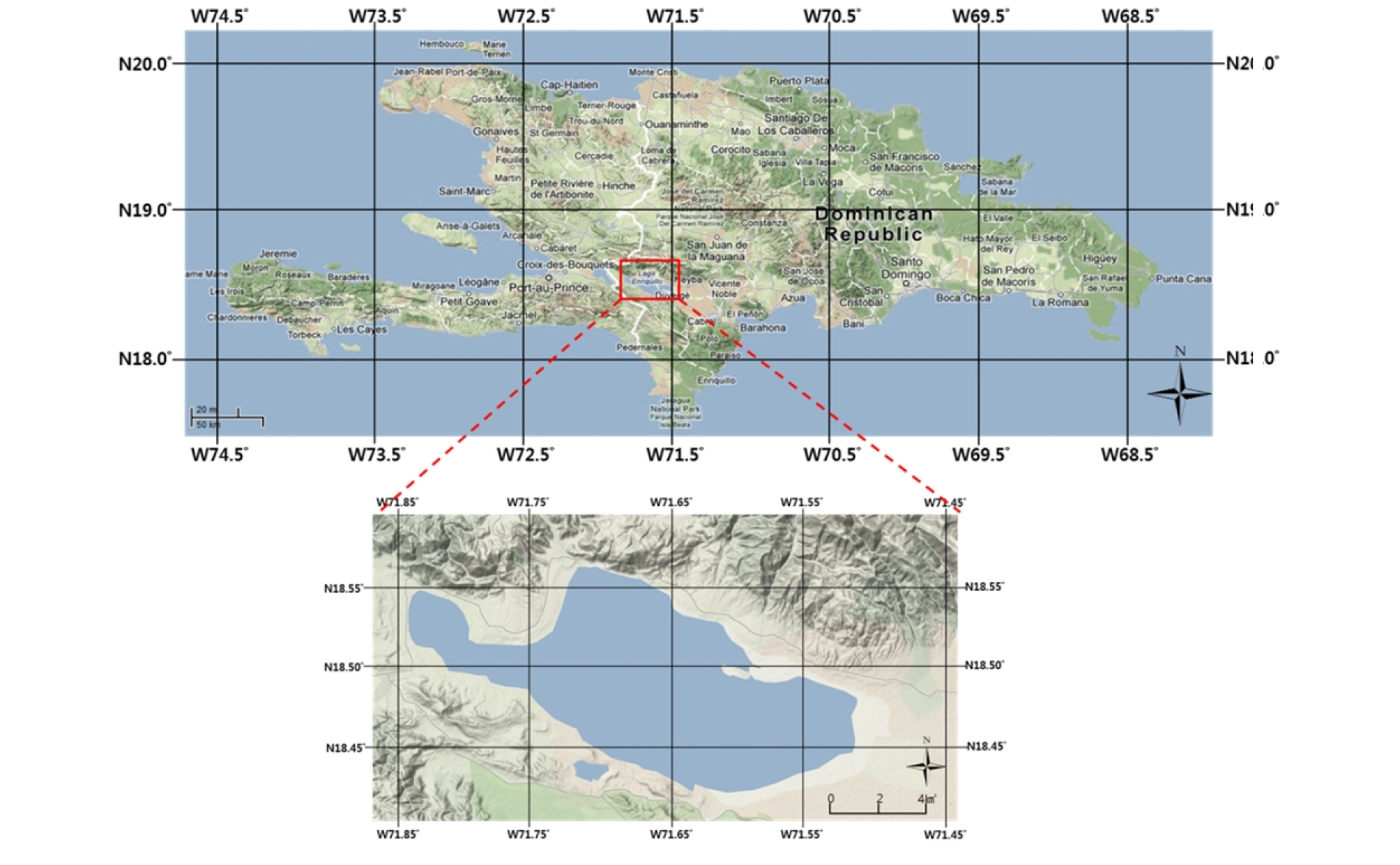
Lake Enriquillo, located in the southwestern region of the Dominican Republic (18°31.7’N, 71°42.91’W), is, with a watershed encompassing about 3750 km², the largest lake in that country and indeed in the entire Caribbean region. Another unique characteristic of the lake is it is also the lowest point in the Caribbean, lying about 45 m below sea level (Buck et al. 2005). The lake region consists of forest, grass, exposed soil, sands, very low-density residential area, and the lake itself. It is bounded by two mountain ranges, Sierra de Neyba to the north and Sierra de Bahoruco to the south, with elevations of about 2,200 m and 1,600 m, respectively (Poteau et al. 2011). The study area is shown in Fig. 1.

Fig. 1.

Lake Enriquillo area.

2.2 Remote sensing data

Terra/MODIS Surface Reflectance 8-day composite L3 Global 500 m (MOD09A1) datasets were selected as the main-data sources in order to monitor the water area of Lake Enriquillo, these datasets, since they are easy to access, free of charge, and offer the best revisit period, represent the best value for each pixel considering 8-day.

MODIS time-series images for each year from 2001 through 2012 were acquired under cloud-free conditions via the USGS MODIS Reprojection Tool Web Interface (MRTWeb). Each MODIS pixel contains the best possible L2G observation made over an 8-day period, as selected on the basis of high observation coverage, a low view angle, the absence of clouds or cloud shadow, and aerosol loading. The MODIS data were registered to Universal Transverse Mercator (Zone 19, North).

Regarding MESMA result validation, we used Landsat-5 TM and Landsat-7 ETM+ images (L1T, path 08 and row 47) of 30 m resolution and six bands (from band 1 to band 7, excluding thermal band 6). They were acquired under cloud-free conditions on 26 December 2002 and on 22 January 2010. The projection information on the Landsat-7 ETM+ data, UTM (Zone 19, North), is the same as MODIS. Table 1 shows acquisition dates of remote sense data that used in this study.

3. Methods

3.1 SMA and MESMA

For classification of images acquired in complex and heterogeneous environments, sub-pixel classification, which presents the strength of membership to each class in a pixel, can be adopted. Sub-pixel analysis, providing a relative abundance of surface materials within a pixel, is preferable to hard classifiers, especially when dealing with satellite sensor data of medium-to-coarse spatial resolution (Myint and Okin 2009). In the numerous studies sub-pixel analysis studies, the linear mixture model (Lu et al. 2003, Smith et al. 1990), background removal spectral mixture analysis (Huguenin et al. 1997), Bayesian probabilities (Myint 2006, Song 2005), neural networks (Foody and Arora 1996, Mertens et al. 2004, Weiguo et al. 2004), fuzzy methods (Fisher and Pathirana 1990, Kumar et al. 2007, Tang et al. 2007, Wang 1990), multivariate statistical analysis (Yang and Liu 2005) and regression tree (Xian 2006) have been applied.

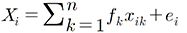
Among all of the sub-pixel analysis approaches, linear spectral mixture analysis (SMA), which provides sub-pixel endmember fraction estimates, probably is the most commonly employed technique (Myint and Okin 2009). SMA models the mixed spectra in the pixels of a remotely sensed image as a combination of the pure spectra of distinct land-surface component endmembers (Adams et al. 1993). SMA is expressed mathematically as Eq. 1:

  (Eq. 1)

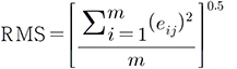
where X_i is the spectral reflectance of band i of a pixel, n is the number of endmembers, f_k is the fraction of an endmember k within a pixel, x_ik is the known spectral reflectance of endmember k within band i, and e_i is the error term for band i. In order to assess the model fit, the root mean square (RMS) error in the equation Eq. 2 is calculated for all pixels, where e_ij is the error term for each of the m spectral bands. The modeled fractions of endmembers are commonly constrained under the “sum to 1” additional condition.

  (Eq. 2)

Despite its popularity, however, SMA fails to account for the existence of materials not included in endmembers or spectral variations in the same material, because it uses fixed endmembers for all pixels in an image (Dennison and Roberts 2003, Pu et al. 2008, Pu et al. 2007).

MESMA, alternatively, is an extension of SMA that addresses the issues of spectral and spatial variability within material classes by allowing the number and type of endmembers to vary on a per-pixel basis. To each pixel, the minimum RMSE model is assigned, producing a fractional image. Model fit is determined by three criteria: the fraction, the RMSE, and the residuals of contiguous bands (Roberts et al. 1998). Thus, by evaluating all possible endmember combinations and selecting the best one for each pixel based on the user-defined criteria, overfitting of a model with too many endmembers can be avoided. MESMA has been utilized in a variety of environment- mapping applications such as vegetation species (Dennison et al. 2000, Roberts et al. 1998), snow grain size (Painter et al. 2003, Painter et al. 1998), marshland (Li et al. 2005), semi-arid land (Okin et al. 2001), urban area (Powell et al. 2007, Rashed 2008, Rashed et al. 2003), water area (Michishita et al. 2012b), minerals (Bedini et al. 2009, Li and Mustard 2003) and fire properties (Dennison et al. 2006, Eckmann et al. 2008).

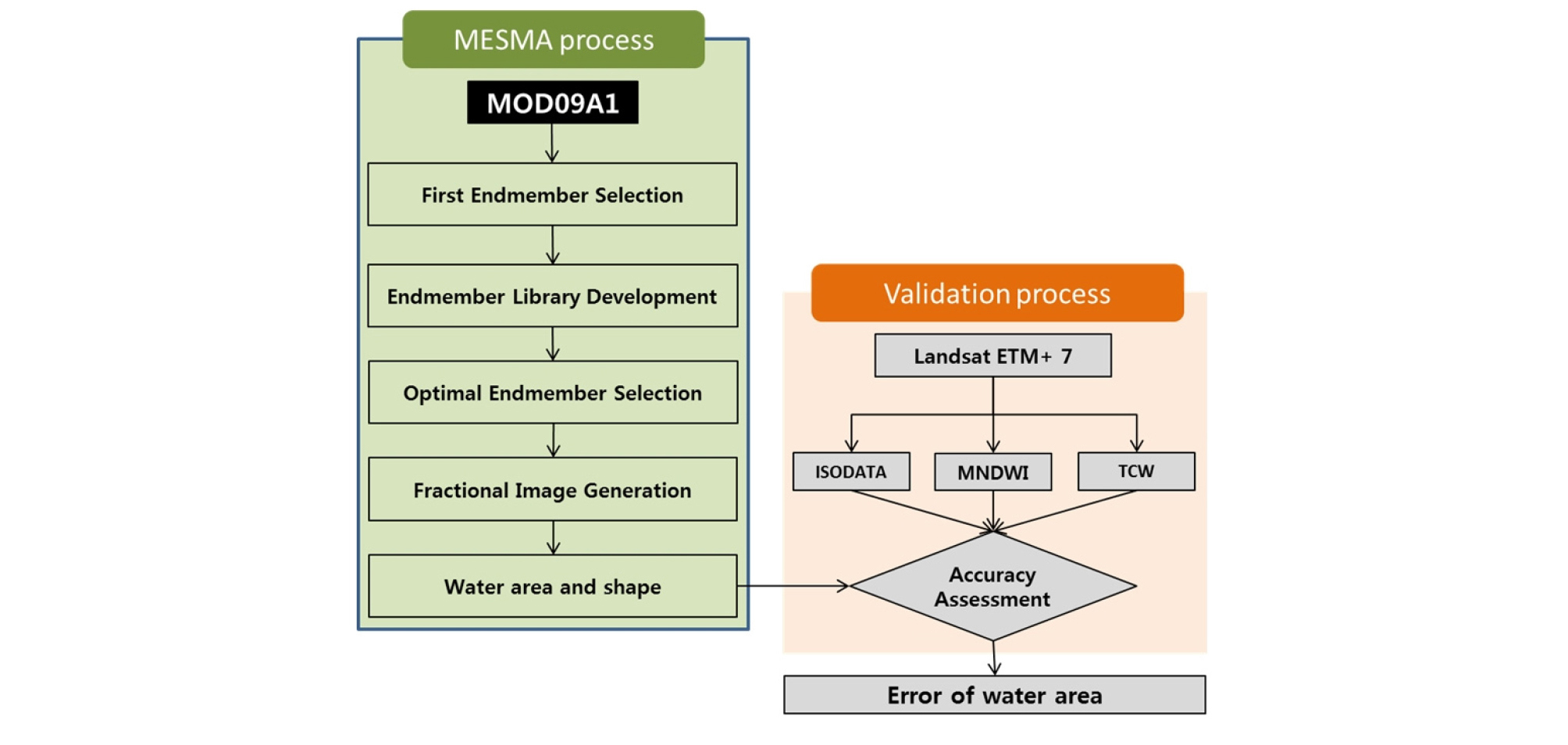
In the present study, MODIS data were used to monitor the variation of the water area of Lake Enriquillo. MODIS offers the advantage of high temporal resolution, though its coarse spatial resolution is a demerit. Fortunately, MESMA can compensate for this, specifically by sub-pixel classification. Moreover, MESMA, as already noted, optimizes each endmember combination for every single pixel. Therefore, MESMA also was utilized in this study. It was implemented with the VIPER Tool (www.vipertools.org), a plug-in software on ENVI. Fig. 2 provides a brief workflow of the algorithms and accuracy assessment used with MESMA in the present research.

Fig. 2.

Workflow of water area extraction.

3.2 First endmember selection and endmember library development

The number of endmember spectra for each class, and definitions of the endmember land-cover classes are other critically important elements in MESMA. Too many endmember spectra cause computation inefficiency and resultant image-interpretation difficulty (Dennison and Robert 2003, Okin et al. 2001). Moreover, as for the representative endmembers, their availability is, generally, highly determinative of the quality of MESMA results (Tompkins et al. 1997). Endmembers can be derived either from image pixels or from a spectral library that contains reference endmembers derived from measurements taken in the field, the laboratory, from radiative transfer models (Sonnentag et al. 2007) or other images. A common technique for determining pure signatures is to select representative pixels from homogeneous land covers in satellite images (Eastman and Laney 2002, Hung and Ridd 2002, Rashed et al. 2003, Small 2001, Wu and Murray 2003).

Some optimal-endmember identification approaches such as Principle Component Analysis (Smith et al. 1985), Simplex (Boardman 1993), and the Pixel Purity Index (PPI) have been developed (Boardman et al. 1995). Using the PPI, pixels from an image are transformed and projected onto a random unit vector. This process, repeated, creates a large number of randomly oriented test vectors anchored at the origin of the coordinate space (Nascimento and Dias 2005). The number of times the pixel is selected as extreme determines its PPI; pixels with high PPIs are then selected as endmembers for multispectral and hyperspectral images. In the present study, we processed the PPI based on the Minimum Noise Fraction (MNF) in order to select the first spectral library. MNF transformation determines the inherent dimensionality of image data, segregates noise, and, thereby, reduces computational requirements. The advantage of implementing MNF into the PPI, specifically, is that it separates purer pixels from more mixed ones, thus reducing the number of pixels to be analyzed and making the separation and identification of endmembers easier (Boardman et al. 1995, De Asis and Omasa 2007).

Concerning three major types of land cover at the study site, about 50 pixels were selected in the MODIS for each endmember type. We refined the selected pixels by visualization of the PPI results, and then, to confirm the endmembers, we geographically linked the PPI images to the MODIS and Landsat-5 TM / Landsat-7 ETM+ band-combination (3/2/1, 4/3/2, 4/5/3) images. Finally, we grouped the endmembers into three classes: soil (exposed soil, sand), vegetation (grass, forest) and shade (water). (For representation of water area by shade, see (Chen and Li 2008, Rashed and Weeks 2003, Rashed et al. 2005).

The endmember library was compiled from the first endmember spectra selections. It was used to assess the variability of the selected endmember spectra and to eliminate outliers. In this way, the final endmember library containing the refined spectra of the selected endmembers was built.

3.3 Optimal endmember selection

Roberts et al. (1998) applied MESMA with all possible two-endmember combinations for a pixel, and, based on user-defined modeling restrictions, determined the optimal mixture model. If a two-endmember combination is satisfactory as a solution, a pixel will be unmixed with it (Michishita et al. 2012b). It also has been found that with the flexible MESMA approach, a majority of pixels in an image can be modeled with only two-endmember combinations. In fact, Powell et al. (2007) determined that natural landscapes in Brazil require only two-endmember models. Franke et al. (2009), additionally, discovered that the two-endmember model effectively discriminates rivers and lakes. Based on these research results, and according to the specific objective of the present study, we used two-endmember combinations to delineate the water area expansion of Lake Enriquillo.

For determination of optimal endmembers, several options, including Endmember Average RMSE (EAR) (Dennison and Roberts 2003), Minimum Average Spectral Angle (MASA) (Dennison et al. 2004), and Count-Based Endmember Selection (CoB) (Rashed et al. 2003), were considered. Adams et al. (1993), Small (2001) and Powell et al. (2007) claimed that EAR is the most effective means of selecting optimal endmember spectra; Michishita et al. (2012b) argued that both EAR and MASA are helpful for choosing strictly defined land-cover types. Based on these findings, we utilized EAR to determine the optimal endmember selection for each image.

In this study, for optimal endmember selection, we used 30 two-endmember models from the endmember library (15 representing soil and 15 representing vegetation). As the second endmember, photometric shade, defined as a spectrum for which the reflectance values of all bands are equal to zero (Adams and Smith 1986), was applied. As two-endmember MESMA modeling constraints, RMSE (0.045), Maximum (1.050), and Minimum (-0.050) fraction, selected based on our analysis of all of the MODIS images, were applied.

3.4 Fraction image generation

Fractional versions of the 11 MODIS images were produced by the 30 two-endmember MESMA models, EAR being utilized to select the optimal two-endmembers for each pixel. The fractional images contained, per pixel, soil (exposed soil, sand), vegetation (grass, forest) and shade (water) land-cover represented by zero or fraction-valued pixels. The zero indicates that a pixel includes only one spectral class within the area that it covers on the ground; the fraction indicates that a pixel includes several spectral classes signifying different types of materials. The shade fractions did not represent an existing land-cover component; they were removed in the normalization process to assess the relative abundance of endmember land cover. Shade normalization divides each non-shade fraction by the sum of all non-shade land-cover classes to produce, in two-endmember models, normalized fractions (Powell et al. 2007).

Once fractional images are generated, the model error has to be checked concerning the number of unclassified pixels and the percent of the overall image information they represent. Since candidate optimal endmembers might not be precisely representative of each land-cover class, a certain amount of unclassified pixel information for fractional images sometimes results. This kind of problem should be resolved by iteratively selecting optimal endmembers and then regenerating the fractional images with the altered MESMA model. This final model could remove error endmembers until no additional improvement could be achieved. We utilized this process to obtain and extract Lake Enriquillo fractional water images from 2001 to 2012.

3.5 Water area calculation

Lake Enriquillo consists of two parts: the water body and the edge area along the shoreline. The total area is calculated based on the fractional water image including zero and fraction-valued pixels. The zero- valued pixels are classified into two groups: 1) those located within the lake area, which is considered as water body; 2) those outside of the lake area, which is considered as noise and excluded from the water area calculation. The fraction-valued pixels also are classified into two groups: 1) those off of the shoreline, which is excluded from the water area calculation; 2) those located along the shoreline, which is considered as edge area. To determine whether or not the pixel belongs to the shoreline, visual inspection with color composites made from three multispectral intervals (Near Infrared, Red, and Green) is performed. After classification, the water area on each pixel is calculated by multiplying the fraction value by the pixel size (250 m by 250 m). Finally, the total water area is obtained by calculating the sum of the water body and edge areas.

4. Results and Discussion

4.1 Accuracy assessment

For validation of the water area in the MODIS- derived MESMA results, we used two reference images which have higher spatial resolution and acquired at the same time as. The first was a Landsat-7 ETM+ image acquired on Dec. 26, 2002, only one month after the MODIS image was obtained (on Nov. 25, 2002). The second was a Landsat-5 TM image acquired on Jan. 22, 2010, about 50 days after the MODIS data acquisition (of Dec. 3, 2009). In order to develop a reference dataset with the Landsat-7 ETM+ image, water area was extracted by three relatively simple, fast and accurate methods: (1) the Modified Normalized Difference Water Index (MNDWI); (2) unsupervised classification (ISODATA), and (3) the tasseled cap wetness (TCW) index. Xu (2006) claimed that MNDWI is more suitable for water area delineation that entails removal of built-up land noise as well as vegetation and soil noise; ISODATA is well known for effective land-cover classification, multispectral water area classification, and noise elimination (Zhang 2000); TCW is used to delineate flood-affected areas immediately before and after a flood (Jain et al. 2005). In this study, water area extracted by the three methods and Landsat images were used to evaluate the accuracy of MESMA’s result, the error of water area (EWA) was thus calculated as shown in Eq. 3.

  (Eq. 3)

Table 2 presents accuracy assessment results which achieved from above steps. The first reference water areas from MNDWI, ISODATA, and TCW using Landsat-7 ETM+ were 169.1 km², 168.2 km², and 171.1 km², respectively, while the fractional water area from MODIS was 168.2 km². The second reference water areas, determined by the same methods but using Landsat-5 TM, were 311.9 km², 309.3 km², and 318.2 km², while the MODIS-derived fractional water area was 310.6 km².

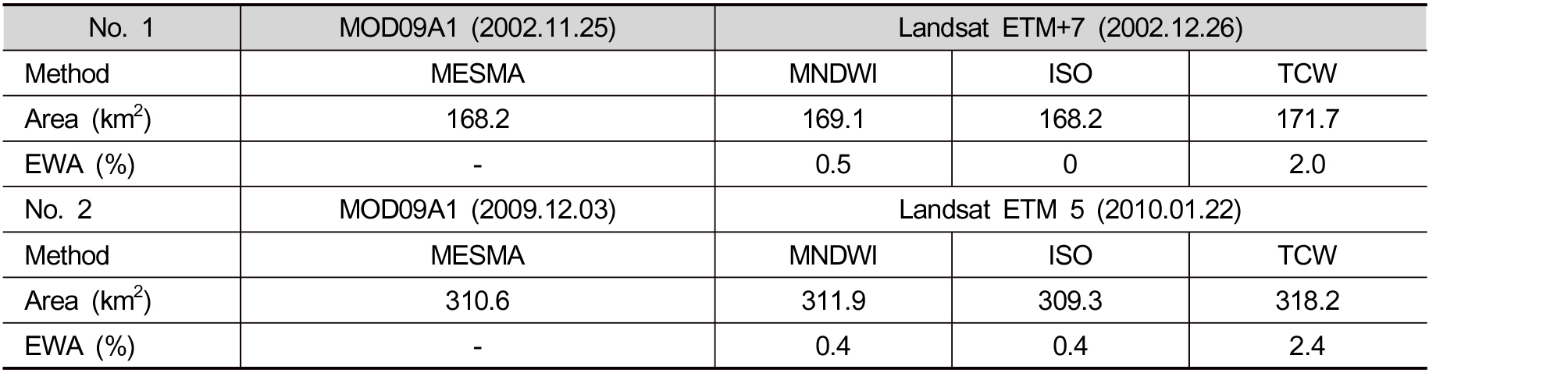
The first EWA values, those between the fractional water area from MODIS and the areas delineated by MNDWI, ISODATA, and TCW from Landsat-7 ETM+, respectively, were 0.5%, 0%, and 2.0%. The second EWA values, those between MODIS and the areas delineated by the same three methods from Landsat-5 TM, respectively, were 0.4%, 0.4%, and 2.4%. These results show that the MODIS-derived fractional water area results by MESMA were very close to those for the processed reference images: approximately 99.1% and 98.9% average accuracies, respectively.

4.2 Spatial expanding patterns of water area changing in lake Enriquillo

The primary objective of this study was to determine, by MESMA, the variation of Lake Enriquillo water area between 2001 and 2012. To explain the spatial patterns of fractional water area, we obtained both RGB image results and MESMA results. Fig. 3 shows the 2001-2012 water fractions which show water expanding trends during the period. As can be seen, the rising of Enriquillo water level can be realized that the peninsula located at western of the lake was developed to the single island from 2001 to 2012; and it seems that the island area has kept its decreasing trend. As for the lake itself, the gradual increases in water area were from the center to the east and west, both areas of low elevation, in contrast to the mountains of the north and south. As for future events, the water area probably will tend to expand more to the east, due to the difference in topographic elevation between the lake and its hydrological basin where consisting of soil, sand, grassland and agricultural land, and due also to the west side is very close to mountainous areas.

Fig. 3.

Fractional images of Lake Enriquillo during 2001 and 2012.

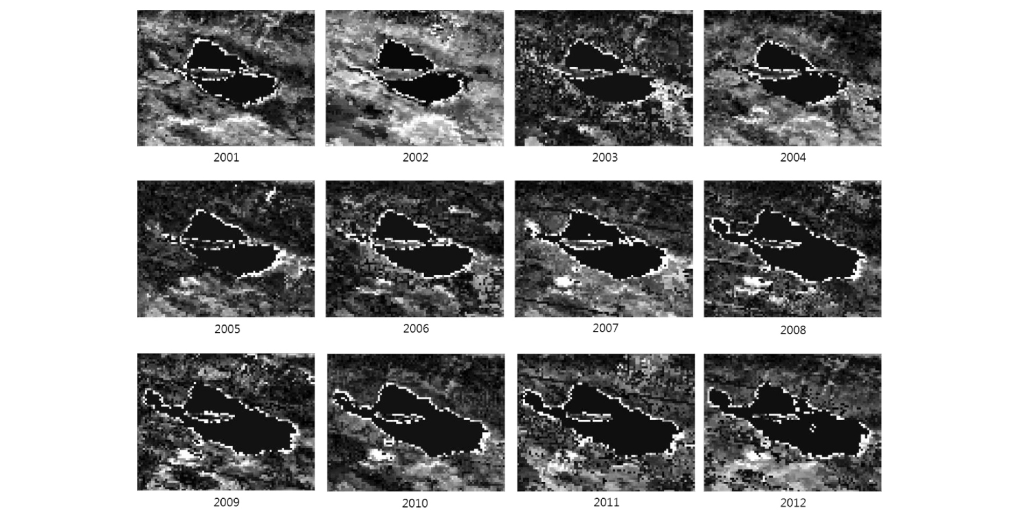
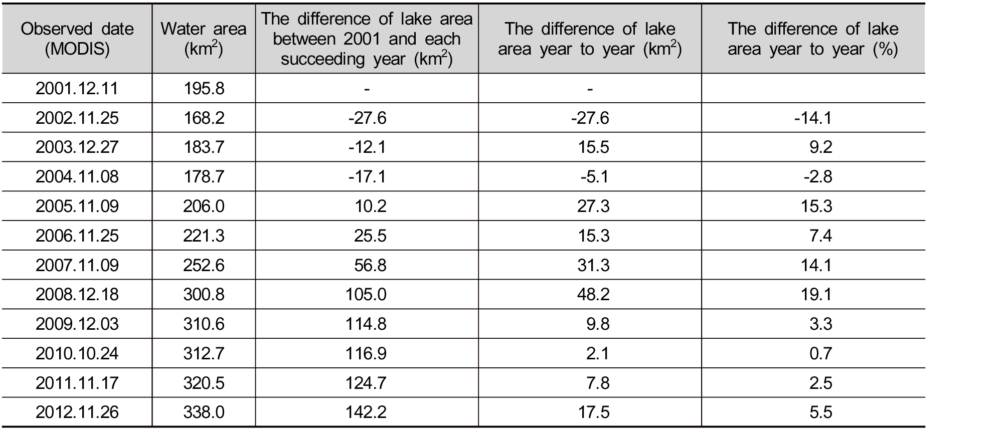
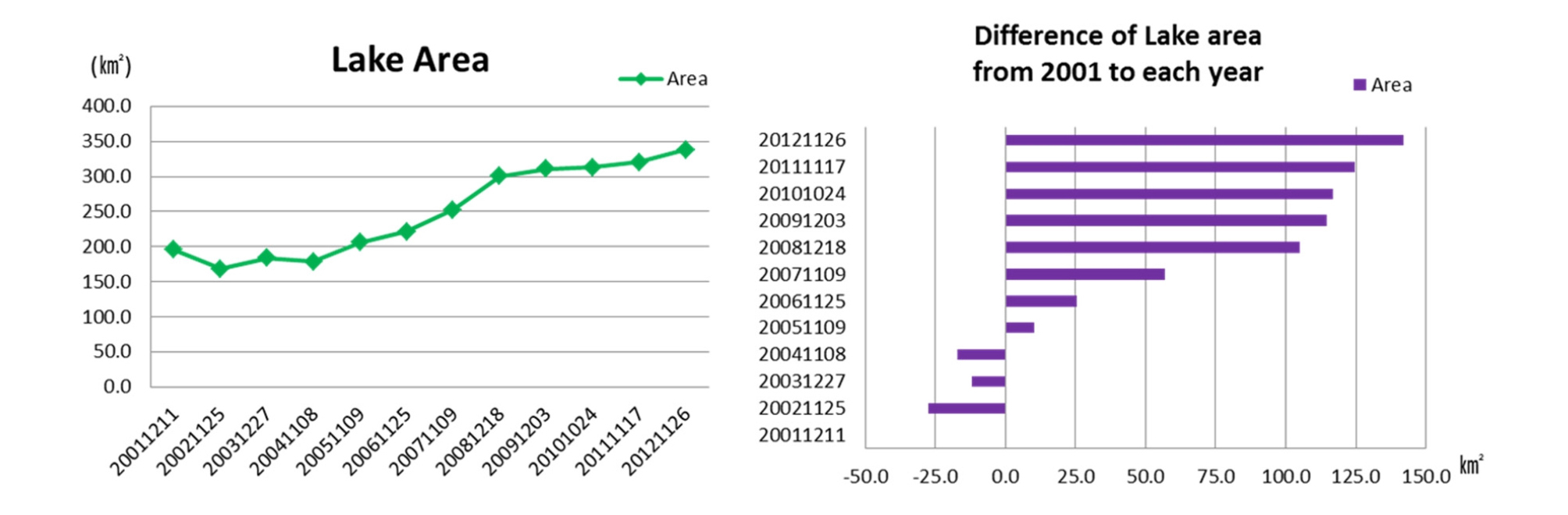
Table 3 and Fig. 4 presents Lake Enriquillo water area changing achieved by MODIS and MESMA. Overall, the Enriquillo size was increased almost double over 12 years, from 195.8 km² to 338.0 km² (an increase of 142.2 km²). However, it experienced a fluctuated period from 2001 to 2004, and its lowest size was 168.2 km² in November 2002. The biggest expending between two continuous years was found 48.2 km², between 2007 and 2008; the second greatest difference was 31.3 km², between 2006 and 2007, while between 2009 and 2010, the water expending rate was just 2.1 km² (0.7%).

Fig. 4.

The difference of lake area between 2001 and each succeeding year.

5. Summary and Conclusions

The design and the results of the present study demonstrate that monitoring and assessment of periodic variation of water area are possible. Specifically, MODIS imaging can be effectively utilized in MESMA delineation of water area. Water area mapping using coarse- spatial-resolution satellite imagery such as MODIS provides challenging due to the mixed-pixel problem. Traditional pixel-based classification with images of this quality typically generates large uncertainties. However, MESMA, based on the concept that any individual spectrum can be modeled with a relatively small number of endmembers, offers a solution to this dilemma. In the present study, we used MESMA to extract water area data in a 2001-2012 time-series and, subsequently on that basis, to map and calculate the dry-season surface water area variation of Lake Enriquillo during those years. In the results, the overall increase in water extent was 142.2 km², and the maximum lake area was 338.0 km² (in 2012). The results of this study show that MESMA effectively generates fractional covers of water area on land. They also suggest the special applicability of MESMA analysis to the identification and assessment of climate-change-effected water variation and potential disaster areas.

Additionally, some hypotheses of lake area change mechanisms were investigated based on the outcomes of the present study, though none of them could fully explain the changes. This fact suggests that further investigations will require monthly water area data.

This will entail the processing of monthly remotely sensed images to isolate the water area expansion from 2004, the year from which the lake has been growing consistently and dramatically; also, the water area fluctuation will be validated using other remote sensing data such as those with a higher spatial resolution from ERS-2 and ENVISAT radar images.