Original Article

Ecology and Resilient Infrastructure. 30 September 2022. 163-173
https://doi.org/10.17820/eri.2022.9.3.163

ABSTRACT


MAIN

  • 1. 서 론

  • 2. 연구 방법

  •   2.1 상세화된 BioClim 구축

  •   2.2 종분포모형 종 출현 자료 구축

  •   2.3 종 생육 특성 및 환경변수 선정

  •   2.4 종분포모형 매개변수 최적화

  • 3. 결과 및 고찰

  •   3.1 모형 성능 및 변수 중요도 평가

  •   3.2 고로쇠나무 잠재 적합 분포 분석

  • 4. 결 론

1. 서 론

IPCC (Intergovernmental Panel on Climate Change, IPCC) 제5차 평가 보고서 (AR5)에 따르면 지구의 평균 온도는 1880 - 2012년 동안 0.85°C가 증가했으며, 1951 - 2012년 사이에만 평균 온도가 0.72°C 증가했다. 온실가스 배출 시나리오의 시뮬레이션에서는 지구 평균 온도가 21세기 말까지 0.3 - 4.8°C가 더 증가하여 지구 온난화가 가속화될 것으로 예상되고 있다 (IPCC 2013, Stocker et al. 2014).

기후변화는 종의 생물계절 (phenology) 및 지리적 분포 변화에 많은 영향을 미치게 되어 종의 멸종 및 번영을 가속화하는 핵심 요인이다 (Parmesan and Yohe 2003, Thomas et al. 2004, Lenoir et al. 2008). 특히 기후는 식생의 분포 패턴을 직접적으로 반영하는 주요 요인으로 (Pounds et al. 2006, Allen and Lendemer 2016), 기후 요인에 대한 정량적인 정보를 취득하고 기후 변화가 잠재적으로 종의 분포에 미치는 영향을 예측하는 연구들이 다수 수행되었다 (Fitzpatrick et al. 2008).

종분포모델 (SDM, species distribution model)은 종과 환경 사이의 관계를 해석하고 결정하기 위한 노력에서 등장했으며 (Guisan and Thuiller 2005, Robertson et al. 2004), 종 분포 데이터의 희소성을 극복하기 위한 좋은 방법 중 하나를 제공한다. SDM은 종의 생태학적 지위 및 반응, 분포 지역 등을 예측하기 위한 입력 자료로 출현/비출현 정보 또는 출현 정보만의 활용 여부나 파라미터의 입력 형식 등의 차이로 GLM (Generalized Linear Model), GAM (Generalized Additive Model), GARP (Genetic Algorithm for Rule-set Production), MaxEnt (Maximum entropy), DOMAIN 등과 같은 다양한 모델들이 개발되었다 (Elith et al. 2006, Guisan et al. 2006, Stockwell 1999, Phillips et al. 2006). 이러한 모델링 방법 중 MaxEnt는 다른 모델링 방법에 비해 작은 샘플 크기에서 더 나은 성능을 발휘하여 희귀종 및 멸종위기종이 잠재 분포를 모델링하는데 효과적이며, 종의 출현 정보만을 가지고도 종의 생태학적 니치를 추정하는 장점이 있어 국내·외에서 널리 사용되고 있다 (Elith et al. 2006, Tsoar et al. 2007)

식생 분포를 예측하는데 가장 영향력 있는 환경 인자는 기후 변수이며 대부분의 연구에서 생태기후지수 (BioClimatic predictor, 이하 BioClim) 자료가 사용되고 있다 (Waltari et al. 2014, Kim et al. 2015, Koo et al. 2016). BioClim은 Worldclim, CliMond, CHELSA 등에서 제공되고 있으나 현재 시기가 각각 다르며, 전지구적 규모로 데이터가 작성되었기 때문에 국내 기후를 잘 반영하는지 검토가 되어야 할 필요가 있다 (Xu and Hutchinson 2011, Kriticos et al. 2012, Karger et al. 2017). 또한, RCP 시나리오 기반의 연구에서는 1 km 해상도로 제공된 WorldClim 자료를 사용할 수 있었으나, Shared Socio-economic Pathways (SSPs) 시나리오에 대해서는 GCM별 미래기간별 기후평균값 이외에 생태기후지수의 값들은 제공되고 있지 않은 실정이다.

1956년 이후 WMO (World Meteorological Organization)는 10년 단위로 30년 기후 평년 (climate normals) 자료를 구축하도록 권고하고 있으며, 30년이라는 단위는 신뢰성 높은 추정치를 산출하기 위한 최적 표본 크기로 알려져 있다 (Arguez and Vose 2011). 우리나라 기상청은 2000년부터 2017년까지 1 km 공간해상도의 기후 자료를 구축하였으나, 관측자료의 시계열이 상대적으로 짧아 장기간 자료에 의한 검증이나 보정이 요구되는 모델링 및 통계적 다운 스케일링 등에 활용하기에 기후 특성을 충분히 반영하지 못하는 것으로 판단된다 (Eum et al. 2018).

본 연구는 상세화된 BioClim 자료의 국내 생태분야에서의 활용을 목적으로 농촌진흥청에서 생산한 1 km 해상도의 SSP 시나리오 기반 상세화 자료를 이용하여 동일한 해상도의 BioClim 생태기후지수 자료를 활용하여 2가지 SSPs 시나리오에 따른 BioClim DB를 구축하고, 이를 종분포모형 기후변화 입력 자료로 활용하여 낙엽활엽교목 고로쇠나무 (Acer pictum subsp. mono (Maxim.) Ohashi)의 분포 변화를 예측하였다.

2. 연구 방법

2.1 상세화된 BioClim 구축

상세화된 BioClim 자료는 O’Donnell1 and Ignizio (2012)가 제시한 20개의 지수를 사용하여 생산되었다. SSPs 시나리오 기반 미래 전망 BioClim 자료를 생산하기 위해서 특정 해상도의 일단위 관측 자료와 동일한 해상도로 가공된 미래 기후변화 상세화 자료가 필요하다. 제공되는 자료는 한반도에 대한 1 km 해상도로 PRISM 기법을 이용하여 생산된 격자 기반 관측 자료와 이를 이용하여, GCM (Global Climate Model)에 대해 동일한 해상도로 생산된 기후변화 상세화 SSPs 시나리오 자료를 입력으로 BioClim 자료를 생산하였다.

SSPs 시나리오는 탄소 중립에 근접한 SSP1-2.6 시나리오와 탄소배출량이 가장 높은 SSP5-8.5 시나리오를 포함하여, SSP2-4.5, SSP3-7.0 등 4개 시나리오를 고려했다. 또한, 미래 전망의 불확실성을 고려하여 18개 GCM을 이용하였으며 (Table 1), 이를 단순 평균한 다중모형앙상블 (MME, Multi-Model Ensemble)로 최종적으로 상세화된 BioClim 자료를 생산했다. MME 기반의 BioClim별 미래 기후변화에 따른 변화 분석은 과거 및 미래 기간에 대해 동일하게 30년 기간에 대한 평균을 계산한 후 비교를 통해 생태지수별 공간적 변화량을 계산하였다. 미래기간은 먼미래 (2071 - 2100년)를 기준으로 30년 기간이 되는 중간미래 (2041 - 2070년) 및 근미래 (2011 - 2040년) 기간을 사용하였다. SSPs 시나리오 자료의 경우 2014년까지를 과거기간 (Historical)으로 사용하고 있으나, 제공된 자료의 경우 과거기간을 1981 - 2010년으로 사용하였다. 과거기간에 대한 재현성 분석은 상세화 자료 생산에 활용된 PRISM 기반 자료를 이용하여 계산된 값과 동일한 과거기간에 대하여 18개 GCM의 평균으로 계산된 값을 비교함으로써 기후모형으로부터 생산된 상세화 자료가 생태지수별 기후특성을 얼마나 잘 재현하는 지를 살펴보았다. 마지막으로 기후변화에 따른 BioClim 생태지수별 미래 전망 변화는 과거기간의 값을 기준으로 미래기간의 값을 비교하여 SSP 시나리오별, 미래 기간별 BioClim 생태지수별 변화의 공간적 분포를 분석하였다.

Table 1.

Produce detailed BioClim data with Multi-Model Ensemble simply averaging 18 GCMs below

Institution (Country) GCMs Resolution References
Geophysical Fluid Dynamics Laboratory (USA) GFDL-ESM4 360×180 John et al. 2018
Meteorological Research Institute (Japan) MRI-ESM2-0 320×160 Yukimoto et al. 2019
Centre National de Recherches
Meteorologiques (France)
CNRM-CM6-1 24572 grids distributed
over 128 latitude circles
Voldoire 2019
CNRM-ESM2-1 Seferian 2019
Institute Pierre-Simon Laplace (France) IPSL-CM6A-LR 144×143 Boucher et al. 2019
Max Planck Institute for Meteorology (Germany) MPI-ESM1-2-HR 384×192 Schupfner et al. 2019
MPI-ESM1-2-LR 192×96 Wieners et al. 2019
Met Office Hadley Centre (UK) UKESM1-0-LL 192×144 Good et al. 2019
Commonwealth Scientific and Industrial Research
Organisation, Australian Research Council Centre of
Excellence for Climate System Science (Australia)
ACCESS-CM2 192×144 Dix et al. 2019
Commonwealth Scientific and Industrial Research
Organisation (Australia)
ACCESS-ESM1-5 192×145 Ziehn et al. 2019
Canadian Centre for Climate Modelling and
Analysis (Canada)
CanESM5 128×64 Swart et al. 2019
Institute for Numerical Mathematics (Russia) INM-CM4-8 180×120 Volodin et al. 2019a
INM-CM5-0 180×120 Volodin et al. 2019b
EC-Earth-Consortium EC-Earth3 512×256 EC-Earth Consortium (EC-Earth) (2019)
Japan Agency for Marine-Earth Science and
Technology/Atmosphere and Ocean Research
Institute/National Institute for Environmental
Studies/RIKEN Center for Computational
Science (Japan)
MIROC6 256×128 Shiogama et al. 2019
MIROC-ES2L 128×64 Tachiiri et al. 2019
NorESM Climate modeling Consortium consisting
of CICERO (Norway)
NorESM2-LM 144×96 Seland et al. 2019
National Institute of Meteorological Sciences/Korea
Meteorological Administration (Korea)
KACE-1-0-G 192×144 Byun et al. 2019

2.2 종분포모형 종 출현 자료 구축

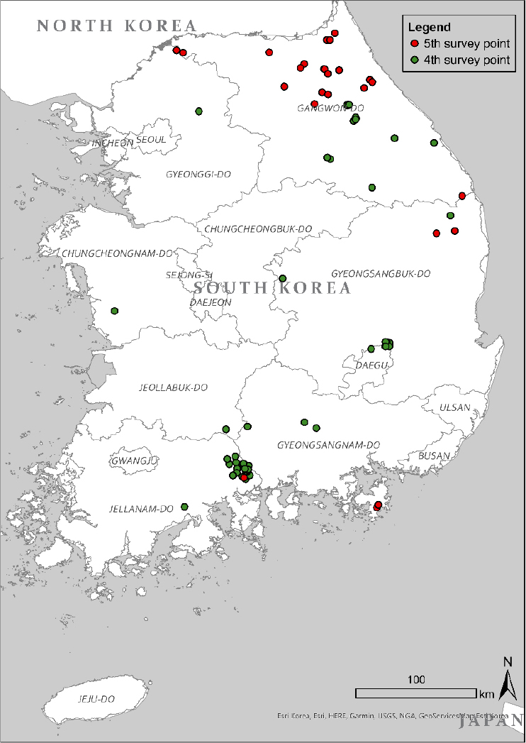
고로쇠나무의 출현 위치 자료는 전국자연환경조사 4차 (2014 - 2018년) 및 5차 일부 (2019 - 2020년) 자료를 통합하여 사용하였다. 4차 조사 자료는 59개 지점으로 전남 광양, 충청, 경북 군위, 강원 남부 일대에서 수집되었으며 5차 조사 자료는 25개 지점으로 경기 북부 및 강원 북부 일대에서 수집된 지점으로 데이터의 수집 시기는 다르지만, 지리적 차이가 확인되어 총 84개 종 발생 지점을 활용했다 (Fig. 1).

https://cdn.apub.kr/journalsite/sites/kseie/2022-009-03/N0190090304/images/kseie_09_03_04_F1.jpg
Fig. 1.

Appearance point of Acer pictum subsp. mono.

2.3 종 생육 특성 및 환경변수 선정

고로쇠나무는 우리나라를 포함한 중국, 일본, 만주 일대에 분포하는 단풍나무과 (Aceraceae) 단풍나무속에 속하는 높이 10 - 30 m의 낙엽활엽교목이다 (Lee et al. 2006). 고로쇠나무는 목재 재질이 단단하여 가구, 악기, 건축 등 자재로 이용되며 국내 건강음료로 활용되는 수종 수액 중 97%가 차지할 정도로 활용 및 보전 가치가 굉장히 높으나 무분별한 벌채 및 수액 채취로 인한 고사 위험에 노출되어 있다 (Song and Hur 2011). 또한 고뢰쇠나무는 이형자웅이숙 (heterodichogamy)의 충매 방법과 검정긴꽃바구미의 종자 가해로 충실 종자 수가 적고, 낙화 후에도 야생동물에 의한 피식 등으로 채종이 어려운 종으로 자연 집단이 점점 소멸되고 있어 있는 실정이다 (Kim et al. 2014).

고로쇠나무는 해발 100 - 1,800 m에서 주로 자생하며 (Lee 1990), 수분 상태가 비교적 양호한 계곡부와 북서사면에 주로 분포하고 있다 (Um and Kim 2006). 따라서 모형에 고로쇠나무의 토양 및 지형적 요인을 반영하기 위해 국토지리정보원에서 제공하는 전국 수치지형도에서 DEM (Digital Elevation Model), 경사 및 향 자료를 구축하였으며, 산림청 산림입지토양도에서 토양 배수 등급도와 지형 유형을 추출하여 변수로 적용했다 (Table 2).

Table 2.

Environment variables entered into the model

Environmental
variables
Description Unit Data type Data soure
Climate Bio01 Annual Mean Temperature °C Continuous Rural Development
Administration-based
SSPs Scenario
Bio02 Mean Diurnal Range °C Continuous
Bio04 Temperature Seasonality °C Continuous
Bio08 Mean Temperature of Wettest Quarter °C Continuous
Bio12 Annual Precipitation mm Continuous
Bio15 Precipitation Seasonality % Continuous
Bio18 Precipitation of Warmest Quarter mm Continuous
Terrain Elevation DEM m Continuous Ministry of Environment,
Korea (2020)
Slope Slope % Continuous
Aspect Aspect ° Continuous
Drainage Soil drainage grade - Categorical Forest Service, Korea
(2020)
Topography Forest Soil Map - Categorical

또한, 식물 생육에 영향을 미치는 기후 자료를 모형 입력 자료로 활용하기 위해 BioClim 18개 기후 인자를 검토하였다. 사례 연구 검토 결과, Hitendra Padali et al. (2017)은 일반적인 기후변화 관점에서 강수량과 기온을 나타내는 Bio01 (연평균 기온)과 Bio12 (연평균 강수량)이 모형 변수로 중요하다고 하였다. 또한 CMIP6의 경우 CMIP5와 비교하여 변동성이 증가한다고 하는데, Bailing and Jian (2014)은 Bio04 (기온 계절성), Bio15 (강수량 계절성), Bio02 (평균 일주 범위), Bio08 (가장 습한 분기의 평균 온도)와 Bio18 (가장 따뜻한 분기의 계절성)이 월단위 및 일단위의 변동성을 잘 설명한다고 강조하여 본 연구에서는 모형 내 입력 자료로 7개 기후 인자를 선정했다. 1차적으로 선정된 변수들 중 다중공선성을 가진 변수를 제거하여 공간자기상관을 확보하기 위해 변수 간 피어슨 상관계수를 확인했으며 r=0.85 이상인 변수는 초기모델 결과에서 기여도가 높은 변수만 남기고 제거했다.

IPCC 6차 평가보고서에서 제공하는 SSP 시나리오 4가지 표준 경로에서 본 연구는 그 중 화석연료 사용 및 기후변화에 따른 고로쇠나무 분포 변화 차이를 가장 크게 확인하고자 SSP1-2.6과 SSP5-8.5 경로 2가지를 확인했다. BioClim 자료는 18개 GCM (Global Climate Model)을 이용하여 단순 평균한 MME 자료를 활용하였으며, 미래 2100년을 기준으로 기준년도 (Hisotrical period, 1981 - 2010년), 근미래 (Near future, 2011 - 2040년), 중간 미래 (Middle future, 2041 - 2070년), 먼미래 (Far future, 2071 - 2100년)의 30년간 평균 자료를 구축했다.

2.4 종분포모형 매개변수 최적화

MaxEnt는 4번의 30년 기간 (기준년도, 근미래, 중간 미래, 먼미래)에 대해 고로쇠나무의 잠재적 적합 분포를 예측하는데 활용되었다. 모델의 예측 성능은 기능 조합 (FC; feature class)과 정규화 승수 (RM; regularization multiplier) 두 가지 매개 변수 선택에 의해 영향을 받는다. FC는 L (linear), Q (quadratic), P (product), T (threshold), H (hinge), C (categorical) 6개 조합으로 모델 최적화가 가능하며, 모델에 사용된 다른 독립변수들의 수학적 변화의 종류를 의미한다 (Elith et al. 2011). RM은 모형에 사용된 FC의 강도를 제어하고 모델 복잡성 및 과적합을 방지한다 (Oh et al. 2021). RM 값이 작을수록 주어진 종 출현 기록에 더 잘 맞는 지역화된 출력 분포가 생성되나 과적합되기 쉬운 경향이 있으며, 반대로 RM 값이 클수록 더 광범위하게 적용할 수 있는 예측을 생성한다. 일반적으로 0.5단계로 등차로 증가시키며 0.5부터 5.0까지 RM 상수 조건을 적용했다. 즉, 6가지 FC (L, H, LQ, LQH, LQPH, LQHPT)와 10가지 RM (0.5, 1.0, 1.5, 2.0, 2.5, 3.0, 3.5, 4.0, 4.5, 5.0)를 적용하여 모형 최적화를 위한 60개 모형 성능을 비교하여 AICc값이 가장 낮은 모형을 선정했다. 일반적으로 낮은 AICc 값이 미래 기후 시나리오를 더 잘 반영하는 것으로 알려져 있다 (Warren and Seifert 2011). 모형 매개변수 최적화를 위해 R 패키지 raster, ENMTools, ENMeval 등을 활용했다.

MaxEnt는 종 출현 지점이 전체적으로 또는 무작위로 일관되게 조사되었다는 것을 기본적인 가정으로 한다 (Kramer-Schadt et al. 2013). 그러나, 실제 종 출현 데이터는 공간적으로 편향되어 있는 우려가 있어 모형 결과가 과적합 (overfitting) 또는 과소적합 (underfitting) 될 수 있다 (Yackulic et al. 2013). 따라서 본 연구에서는 종 발생 지점 좌표를 기반으로 2차원 커널 밀도 추정치를 제공하는 R 패키지 MASS의 kde2d 함수를 사용하여 bias layer를 생성하고 모델에 적용하여 출력의 과적합을 방지했다. MaxEnt의 ‘Replicates’는 10회, ‘Replicated run type’은 ‘Crossvalidate’로 선택하였으며, 모형에서 사용 가능한 잠재적인 배경 지점이 약 38,000개로 확인되어 ‘Max number of background points’는 일반적으로 배경 지점이 10,000개 이상이면 10,000으로 설정하기 때문에 10,000으로 설정했다 (Barbet-Massin et al. 2012).

모형의 예측 정확도는 AUC 값에 따라 5개의 등급 (fail : 0.5 - 0.6, poor: 0.6 - 0.7, fair: 0.7 - 0.8, good: 0.8 - 0.9, excellent: 0.9 - 1.0)으로 분류했다 (Swets 1988). 변수의 중요성은 기여도 (Percent Contribution)와 중요도 (Permutation Importance)를 통해 확인했고, 변수 간 중요도는 Jackknife 검정을 수행하여 확인했다. 또한, 변수별 반응곡선을 확인하여 분포확률과의 관계를 확인했다. 마지막으로 종의 잠재적인 분포 영역을 평가하기 위해 MaxEnt 결과로 도출된 적합도는 기후변화에 따른 서식 적합성 평가 시 보편적으로 사용하는 등간격 접근법인 ‘equal interval approach’를 사용하여 5가지 등급 (0 - 0.2, 부적합; 0.2 - 0.4, 낮은 적합성; 0.4 - 0.6, 일반 적합성; 0.6 - 0.8, 중간 적합성; 및 0.8 - 1, 높은 적합성)으로 적합한 분포 지역을 분류했다 (Li et al. 2020, Ab Lah et al. 2021).

3. 결과 및 고찰

3.1 모형 성능 및 변수 중요도 평가

1차로 선정된 환경 변수 간 0.85 이상 상관성이 확인되지 않아, 최종 모델 구동에도 동일하게 5개의 지형 변수와 7개의 기후 변수를 활용했다. 모형 성능 결과는 RM 값 1.5과 함께 FC 값 LQH를 선택하는 ‘LQH-1.5’가 최적의 성능 모형을 제공하는 것으로 나타났다. LQH-1.5 모델을 이용하여 7개의 고로쇠나무 잠재 분포 지역을 예측한 결과, 모형의 평균 test AUC 값은 0.881로 예측 정확도가 높고, 신뢰할 수 있는 적합한 모형이라 해석되었다 (Fig. 2).

국내 고로쇠나무 분포에 있어 높은 기여도를 나타내는 변수는 배수 등급 (26.9%)과 Bio12 (23.8%), 경사(23.0%), Bio08 (11.2%), 고도 (9.1%) 순으로 확인되었으며, 변수 중요도는 bio12 (31.7%), bio08 (28.0%), 경사 (17.6%), 배수 등급 (13.8%), 고도 (3.0%) 순으로 확인되었다 (Fig. 2, Table 3).
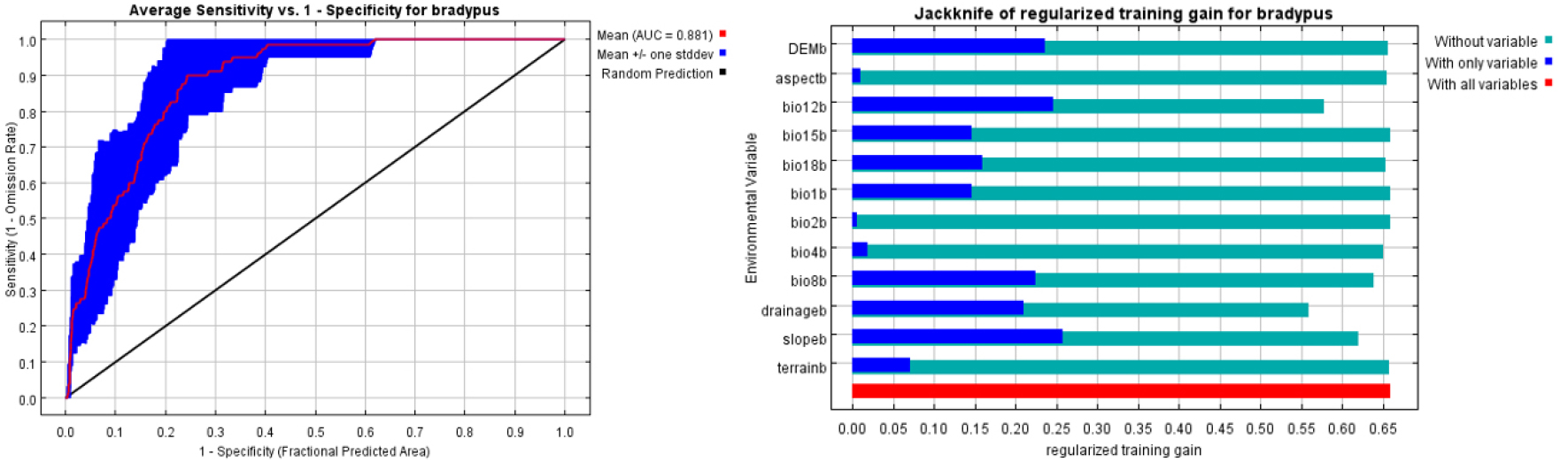
https://cdn.apub.kr/journalsite/sites/kseie/2022-009-03/N0190090304/images/kseie_09_03_04_F2.jpg
Fig. 2.

Jackknife test of regularized training gain contribution of the considered environmental variables and their.

Table 3.

Contribution and importance between climate and terrain variables in MaxEnt

Variable Percent contribution Permutation importance
drainage 26.9 13.8
bio12 23.8 31.7
slope 23 17.6
bio8 11.2 28
DEM 9.1 3

기여도가 높은 주요 변수에 대한 반응 곡선을 확인한 결과, 배수 5등급, Bio12 (연평균 강수량)이 2,250 mm 이상, 경사는 10 - 20°, Bio08 (가장 습한 분기의 평균 온도)가 15°C 이하, 고도는 높을수록 고로쇠나무 분포에 긍정적인 영향을 미치는 것으로 해석되었다 (Fig. 3).

https://cdn.apub.kr/journalsite/sites/kseie/2022-009-03/N0190090304/images/kseie_09_03_04_F3.jpg
Fig. 3.

Response curves for key variables in MaxEnt results.

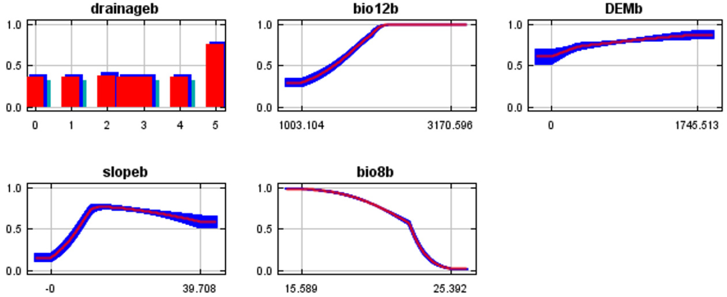
분석 결과는 고로쇠나무는 배수, 강수량 등 기온보다는 습윤 상태가 생육에 가장 중요하게 확인되었으며, 이는 국내 분포하는 고로쇠나무가 토양 A층에 적습하고 비옥한 토양을 선호하는 것으로 알려져 있는 것과 동일한 분석 결과이다 (Um and Kim 2006). 또한 반대로, 모델 분석 결과 고로쇠나무 생육에는 기온 요인이 크게 작용하지 않는 것으로 보아, 본 모델에 적용한 상세화된 BioClim 기후 변수가 국내 기후를 잘 반영한 결과라 해석할 수 있다.

3.2 고로쇠나무 잠재 적합 분포 분석

기준년도로 확인된 고로쇠나무의 적합 분포 지역은 남해안과 동해안, 강원 북부 지역을 따라 실제 분포와 유사하였다. 실제 고로쇠나무의 출현 지점 이외에도 월악산-속리산-덕유산-가야산을 잇는 백두대간 일대에서도 적합한 분포 지역으로 확인되었다 (Fig. 4). 전국자연환경조사에서 확인된 고로쇠나무 분포 지점과 기준년도 고로쇠나무 잠재 적합 분포 지도를 비교한 결과, 평균 0.599 (±0.139)로 확인되었다. 기준년도에서 고로쇠나무의 적합성 비율은 높은 적합성 3.41%, 중간 적합성 7.97%, 일반 적합성 11.23%, 낮은 적합성 19.54%, 부적합 57.83%로 확인되었다. 국토 면적 대비 대부분 고로쇠나무의 생육이 적합하지 않은 것으로 확인되었다.

https://cdn.apub.kr/journalsite/sites/kseie/2022-009-03/N0190090304/images/kseie_09_03_04_F4.jpg
Fig. 4.

Potential distribution of suitable area of Acer pictum subsp. mono under climate change using SSP1-2.6 and SSP5-8.5 in South Korea.

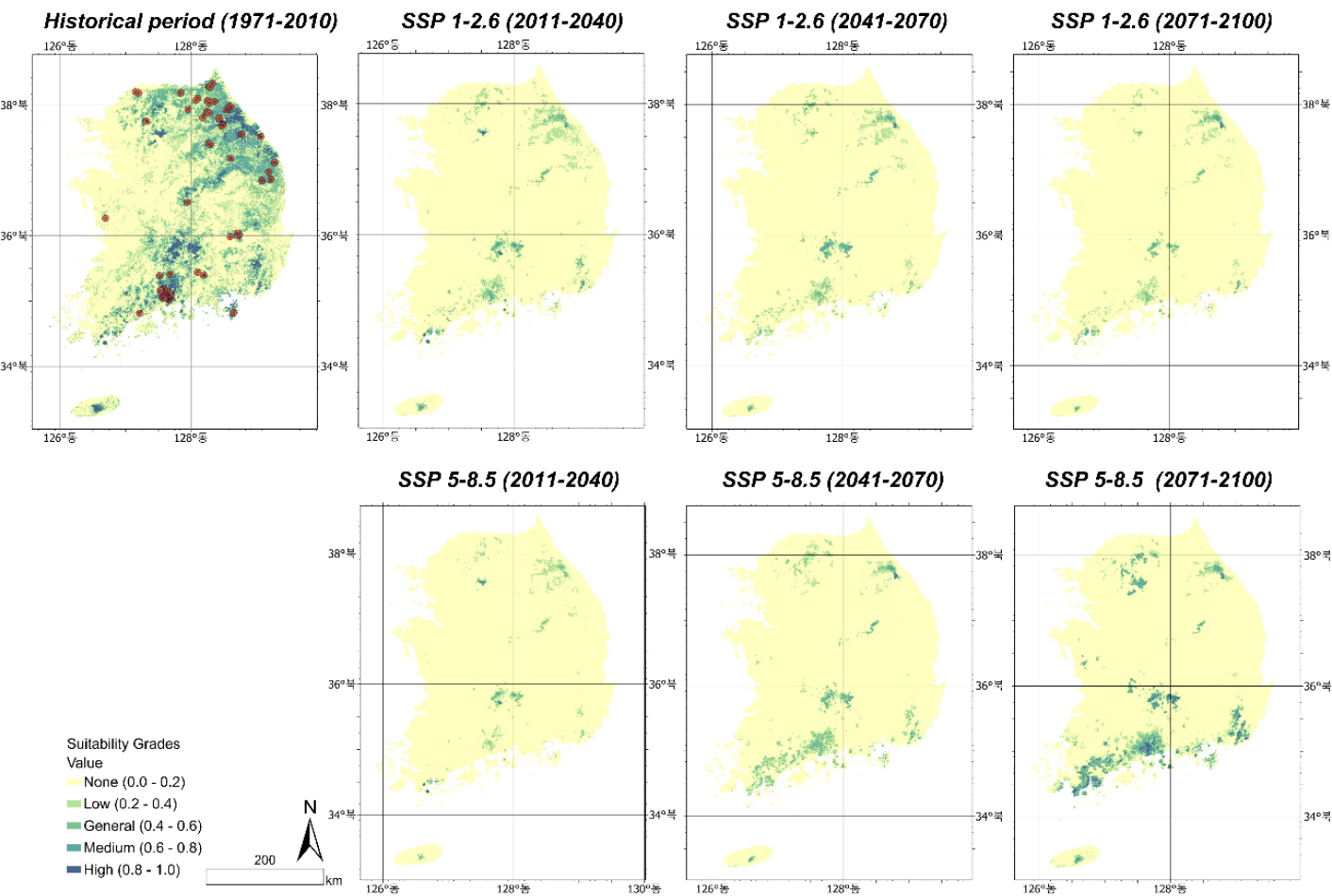
기준년도 고로쇠나무의 적합 분포 지도에 미래 기후변화 시나리오 SSP1-2.6과 SSP5-8.5를 투영한 결과, 미래 고로쇠나무 잠재 분포 지역이 현저하게 감소하는 것으로 확인되었다. SSP1-2.6 근미래에 고로쇠나무 우수 적합 비율이 0.10%, 중간 미래에는 0.02%, 먼미래에는 0.02%까지 감소하여 온실가스 저배출로 인해 대기 온도가 약 1.2 - 2.4°C만 증가하더라도 강수량 등 다른 환경 조건이 적합하지 않아 국내에서 잠재 분포 지역이 지속적으로 감소하는 것으로 예측되었다 (Arias et al. 2021). 반면에 SSP5-8.5에서는 고로쇠나무 적합 비율이 근미래에 0.01%, 중간 미래에 0.01%, 먼미래에 0.72%로 확인되어, 기준년대 대비 중간 미래까지 생육지 비율이 감소했으나 SSP1-2.6 시나리오와는 반대로 먼미래로 갈수록 남부 해안가와 경기 북동부 및 고도가 높은 지리산-덕유산-가야산 국립공원을 중심으로 고로쇠나무 생육 조건이 적합해지는 것으로 예측되었다. 이는 SSP5-8.5 시나리오에서 먼 미래로 갈수록 소백산맥의 높은 고도 지대와 남부지역 및 경기 북동부 지역의 연평균 강수량이 증가함이 반영된 결과라 할 수 있다.

따라서 고로쇠나무는 2가지의 상세화된 기후 시나리오를 반영했을 때 현재 위치와 비교하여 기후 변화와 관계없이 대부분의 적합 분포 지역이 감소하는 것으로 확인되었으며, Bio12 기후 인자에 의한 연 평균 강수량이 약 2,000 mm 이상 유지되는 것이 모델 결과에 반영된 것으로 해석된다. 고로쇠나무가 온도 영향보다는 강수량 등 서식지 습윤 상태에 더 민감하여 개발과 탄소 배출이 확대되는 시나리오에서 서식이 더 양호할 것으로 예측되었다. 그러나 국내 고로쇠나무의 온량 지수가 28-121°C로 알려져 있어, 기후변화에 대한 유연성이 크다고 할 수 있으나, 상세화된 SSP5-8.5 시나리오에서 대기 온도가 약 1.6°C부터 최대 4.4°C까지 상승하기 때문에 생육 가능한 온량 지수 임계값을 넘어 급격한 온도 변화는 고로쇠나무의 생육에 부정적 영향을 미칠 것으로 해석된다 (Korea Forest Service 2022).

4. 결 론

기후변화는 종의 지리적 분포 변화에 많은 영향을 미치게 되어 종의 멸종을 가속화하는 핵심 요인이다. 그러나 생물의 생리적 특성을 반영하여 입력자료로 종분포모델에 적용되는 BioClim의 경우, 우리나라 여건이 반영되지 않은 WorldClim 자료가 활용되고 있어 모델 결과에 대한 불확실성이 높다. 본 연구는 농촌진흥청에서 제작한 SSP 시나리오 기반 BioClim 상세화 자료를 이용하여 국내 고로쇠나무 서식지의 분포 변화 양상을 파악했다. 고로쇠나무는 7개의 상세화된 기후 변수와 5개의 지형 변수 중 강수량과 토양의 배수 능력에 가장 많은 영향을 받는 것으로 확인되었다. 이는 고로쇠나무가 토양 A층이 비옥하고 습한 지역에서 서식하는 특성을 반영한 결과로 해석된다.

본 연구는 국내 여건을 고려한 기후변화 상세화 시나리오를 기반으로 제작된 BioClim 자료를 활용하여 고로쇠나무의 미래 서식 변화 양상을 확인한 연구로, 특히 MaxEnt 모형의 구동 불확실성을 줄이기 위해 모형의 다양한 조건을 고려하여 도출한 결과로서 의의가 있다. 이를 통해 국내 서식하는 고로쇠나무가 기온 변화 외에 강수량 변동성도 종 출현에 주된 영향을 줄 수 있다는 가능성을 확인하였다. 또한, 탄소배출이 확대되어 식물종의 서식 감소가 필연적으로 발생하는 연구의 시각이 아닌, 오히려 기후 변화에 보다 적응이 수월한 종이 미래 분포 양상을 확인한 새로운 시각의 연구가 될 수 있으며, 기후 변화 적응 종으로서 미래 산림 복원 등에 활용 가능한 기초 연구로서 의의가 있다.

Acknowledgements

이 연구는 농촌진흥청 “신농업기후변화대응체계구축사업 (과제번호: PJ015576)”의 지원으로 수행되었습니다.

References

1
Ab Lah, N. Z., Yusop, Z., Hashim, M., Mohd Salim, J., and Numata, S. 2021. Predicting the Habitat Suitability of Melaleuca cajuputi Based on the MaxEnt Species Distribution Model. Forests 12(11): 1449. 10.3390/f12111449
2
Allen, J.L. and Lendemer, J.C. 2016. Climate change impacts on endemic, high-elevation lichens in a biodiversity hotspot. Biodiversity and Conservation 25(3): 555-568. 10.1007/s10531-016-1071-4
3
Arguez, A. and Vose, R.S. 2011. The definition of the standard WMO climate normal: The key to deriving alternative climate normals. Bulletin of the American Meteorological Society 92(6): 699-704. 10.1175/2010BAMS2955.1
4
Arias, P., Bellouin, N., Coppola, E., Jones, R., Krinner, G., Marotzke, J., ... and Zickfeld, K. 2021. Climate Change 2021: The Physical Science Basis. Contribution of Working Group14 I to the Sixth Assessment Report of the Intergovernmental Panel on Climate Change; Technical Summary.
5
Bailing, M. and Jian, S. 2018. Predicting the distribution of Stipa purpurea across the Tibetan Plateau via the MaxEnt model. BMC Ecology 18(1): 1-12. 10.1186/s12898-018-0165-029466976PMC5822641
6
Barbet-Massin, M., Jiguet, F., Albert, C.H., and Thuiller, W. 2012. Selecting pseudo‐absences for species distribution models: how, where and how many?. Methods in ecology and evolution 3(2): 327-338. 10.1111/j.2041-210X.2011.00172.x
7
Boucher, O., Denvil, S., Levavasseur, G., Cozic, A., Caubel, A., Foujols, M.A., Meurdesoif, Y., Cadule, P., Devilliers, M., Dupont, E., and Lurton, T. 2019. IPSL IPSL-CM6A-LR model output prepared for CMIP6 ScenarioMIP. Earth System Grid Federation. https://doi.org/10.22033/ESGF/CMIP6.1532 .
8
Byun, Y.H., Lim, Y.J., Shim, S., Sung, H.M., Sun, M., Kim, J., ... and Moon, H. 2019. NIMS-KMA KACE1. 0-G model output prepared for CMIP6 ScenarioMIP. Earth System Grid Federation.
9
Dix, M., Bi, D., Dobrohotoff, P., Fiedler, R., Harman, I., Law, R., Mackallah, C., Marsland, S., O'Farrell, S., Rashid, H., Srbinovsky, J., Sullivan, A., Trenham, C., Vohralik, P., Watterson, I., Williams, G., Woodhouse, M., Bodman, R., Dias, F. B., … and Yang, R. 2019. CSIRO-ARCCSS ACCESS-CM2 model output prepared for CMIP6 ScenarioMIP. Earth System Grid Federation. 10.22033/ESGF/CMIP6.2285.
10
EC-Earth Consortium (EC-Earth). 2019. EC-Earth-Consortium EC-Earth3 model output prepared for CMIP6 ScenarioMIP. Earth System Grid Federation. https://doi.org/10.22033/ESGF/CMIP6.251 .
11
Elith, J., Graham, H.C., Anderson, P.R., Dudík, M., Ferrier, S., Guisan, A., ... and Zimmermann, E.N. 2006. Novel methods improve prediction of species' distributions from occurrence data. Ecography 29(2): 129-151. 10.1111/j.2006.0906-7590.04596.x
12
Elith, J., Phillips, S.J., Hastie, T., Dudík, M., Chee, Y. E., and Yates, C.J. 2011. A statistical explanation of MaxEnt for ecologists. Diversity and distributions 17(1): 43-57. 10.1111/j.1472-4642.2010.00725.x
13
Eum, H.I., Kim, J.P., and Cho, J. 2018. High-resolution climate data from an improved GIS-based regression technique for South Korea. KSCE Journal of Civil Engineering 22(12): 5215-5228. (in Korean) 10.1007/s12205-017-1441-9
14
Fitzpatrick, M.C., Gove, A.D., Sanders, N.J., and Dunn, R.R. 2008. Climate change, plant migration, and range collapse in a global biodiversity hotspot: the Banksia (Proteaceae) of Western Australia. Global Change Biology 14(6): 1337-1352. 10.1111/j.1365-2486.2008.01559.x
15
Good, P., Sellar, A., Tang, Y., Rumbold, S., Ellis, R., Kelley, D., Kuhlbrodt, T., and Walton, J. 2019. MOHC UKESM1.0-LL model output prepared for CMIP6 ScenarioMIP. Earth System Grid Federation. 10.22033/ESGF/CMIP6.1567.
16
Guisan, A. and Thuiller, W. 2005. Predicting species distribution: offering more than simple habitat models. Ecology letters 8(9): 993-1009. 10.1111/j.1461-0248.2005.00792.x34517687
17
Guisan, A., Lehmann, A., Ferrier, S., Austin, M., Overton, J.M.C., Aspinall, R., and Hastie, T. 2006. Making better biogeographical predictions of species' distributions. Journal of Applied Ecology 43(3): 386-392. 10.1111/j.1365-2664.2006.01164.x
18
IPCC, A. 2013. Climate change 2013: the physical science basis. Contribution of working group I to the fifth assessment report of the intergovernmental panel on climate change 1535.
19
John, J.G., Blanton, C., McHugh, C., Radhakrishnan, A., Rand, K., Vahlenkamp, H., ... and Zeng, Y. 2018. Noaa-gfdl gfdl-esm4 model output prepared for cmip6 scenariomip. Earth System Grid Federation.
20
Karger, D.N., Conrad, O., Böhner, J., Kawohl, T., Kreft, H., Soria-Auza, R.W., ... and Kessler, M. 2017. Climatologies at high resolution for the earth's land surface areas. Scientific data 4(1): 1-20. 10.1038/sdata.2017.12228872642PMC5584396
21
Kim, G.T., Kim, H.J., and Lee, J.H. 2014. Studies on the Community Structure, Samara and Leaf Shape of Three Natural Acer pictum subsp. mono Forest. Korean Journal of Environment and Ecology 28(1): 55-61. (in Korean) 10.13047/KJEE.2014.28.1.55
22
Kim, J., Jung, H., Jeon, S.W., and Lee, D.K. 2015. Predicting the potential distribution of Korean pine (Pinus koraiensis) using an ensemble of climate scenarios. Journal of the Korean Society of Environmental Restoration Technology 18(2): 79-88. (in Korean) 10.13087/kosert.2015.18.2.79
23
Koo, K.A., Kim, J., Kong, W.S., Jung, H., and Kim, G. 2016. Projecting the potential distribution of Abies koreana in Korea under the climate change based on RCP scenarios. Journal of the Korean Society of Environmental Restoration Technology 19(6): 19-30. (in Korean) 10.13087/kosert.2016.19.6.19
24
Kramer-Schadt, S., Niedballa, J., Pilgrim, J.D., Schröder, B., Lindenborn, J., Reinfelder, V., ... and Wilting, A. 2013. The importance of correcting for sampling bias in MaxEnt species distribution models. Diversity and distributions 19(11): 1366-1379. 10.1111/ddi.12096
25
Kriticos, D.J., Webber, B.L., Leriche, A., Ota, N., Macadam, I., Bathols, J., and Scott, J.K. 2012. CliMond: global high‐resolution historical and future scenario climate surfaces for bioclimatic modelling. Methods in Ecology and Evolution 3(1): 53-64. 10.1111/j.2041-210X.2011.00134.x
26
Lee, B., Chung, J., and Kwon, D.S. 2006. Analysis of site suitability of forest stands for extracting sap of Acer pictum var. mono using GIS and fuzzy sets. Journal of Korean Society of Forest Science 95(1): 38-44. (in Korean)
27
Lee, C.B. 1990. Dendrology. Hangmoon Pub. Co., Seoul, Korea, 253.
28
Lenoir, J., Gégout, J. C., Marquet, P.A., de Ruffray, P., and Brisse, H. 2008. A significant upward shift in plant species optimum elevation during the 20th century. Science 320(5884): 1768-1771. 10.1126/science.115683118583610
29
Li, Y., Li, M., Li, C., and Liu, Z. 2020. Optimized maxent model predictions of climate change impacts on the suitable distribution of cunninghamia lanceolata in China. Forests 11(3): 302. 10.3390/f11030302
30
O'Donnell, M.S., and Ignizio, D.A. 2012. Bioclimatic predictors for supporting ecological applications in the conterminous United States. US Geological Survey Data Series 691(10): 4-9. 10.3133/ds691
31
Oh, Y.J., Kim, M.H., Choi, S.K., Kim, M.K., Eo, J., Yeob, S.J., ... and Lee, Y.H. 2021. Prediction of the spatial distribution of suitable habitats for Geranium carolinianum under SSP scenarios. Ecology and Resilient Infrastructure 8(3): 154-163. (in Korean)
32
Parmesan, C. and Yohe, G. 2003. A globally coherent fingerprint of climate change impacts across natural systems. Nature 421(6918): 37-42. 10.1038/nature0128612511946
33
Phillips, S.J., Anderson, R.P., and Schapire, R.E. 2006. Maximum entropy modeling of species geographic distributions. Ecological Modelling 190(3-4): 231-259. 10.1016/j.ecolmodel.2005.03.026
34
Pounds, J.A., Bustamante, M.R., Coloma, L.A., Consuegra, J.A., Fogden, M.P., Foster, P.N., ... and Young, B.E. 2006. Widespread amphibian extinctions from epidemic disease driven by global warming. Nature 439(7073): 161-167. 10.1038/nature0424616407945
35
Robertson, M.P., Villet, M.H., and Palmer, A.R. 2004. A fuzzy classification technique for predicting species' distributions: applications using invasive alien plants and indigenous insects. Diversity and Distributions 10(5-6): 461-474. 10.1111/j.1366-9516.2004.00108.x
36
Seferian, R. 2019. CNRM-CERFACS CNRM-ESM2-1 model output prepared for CMIP6 ScenarioMIP. Earth System Grid Federation. 10.22033/ESGF/CMIP6,1395.
37
Seland, Ø., Bentsen, M., Oliviè, D.J.L., Toniazzo, T., Gjermundsen, A., Graff, L.S., ... and Schulz, M. 2019. NCC NorESM2-LM model output prepared for CMIP6 ScenarioMIP. Earth System Grid Federation. https://doi.org/10.22033/ESGF/CMIP6.604 .
38
Shiogama, H., Abe, M., and Tatebe, H. 2019. MIROC MIROC6 model output prepared for CMIP6 ScenarioMIP. Earth System Grid Federation.
39
Song, J.H. and Hur, S.D. 2011. Analysis of leaf morphological variation of 11 natural populations of Acer pictum subsp. mono (Maxim.) Ohashi. Korean Journal of Plant Resources 24(5): 540-548. (in Korean) 10.7732/kjpr.2011.24.5.540
40
Stocker, T. (Ed.). 2014. Climate change 2013: the physical science basis: Working Group I contribution to the Fifth assessment report of the Intergovernmental Panel on Climate Change. Cambridge university press.
41
Stockwell, D. 1999. The GARP modelling system: problems and solutions to automated spatial prediction. International Journal of Geographical Information Science 13(2): 143-158. 10.1080/136588199241391
42
Swart, N.C., Cole, J.N., Kharin, V.V., Lazare, M., Scinocca, J.F., Gillett, N.P., ... and Sigmond, M. 2019. CCCma CanESM5 model output prepared for CMIP6 ScenarioMIP. Earth System Grid Federation.
43
Swets, J.A. 1988. Measuring the accuracy of diagnostic systems. Science, 240(4857): 1285-1293. 10.1126/science.32876153287615
44
Tachiiri, K., Abe, M., Hajima, T., Arakawa, O., Suzuki, T., Komuro, Y., ... and Kawamiya, M. 2019. MIROC MIROC-ES2L model output prepared for CMIP6 ScenarioMIP. Earth System Grid Federation. Retrieved from http://cera-www.dkrz.de/WDCC/meta/CMIP6/CMIP6.ScenarioMIP.MIROC.MIROC-ES2L .
45
Thomas, C.D., Cameron, A., Green, R.E., Bakkenes, M., Beaumont, L.J., Collingham, Y.C., ... and Williams, S. E. 2004. Extinction risk from climate change. Nature 427(6970): 145-148. 10.1038/nature0212114712274
46
Tsoar, A., Allouche, O., Steinitz, O., Rotem, D., and Kadmon, R. 2007. A comparative evaluation of presence- only methods for modelling species distribution. Diversity and distributions 13(4): 397-405. 10.1111/j.1472-4642.2007.00346.x
47
Um, T.W. and Kim, G.T. 2006. Distribution and growth characteristics of Acer pictum var. mono in relation to topography and soil in Mt. Joongwang, Gangwon Province. Korean Journal of Environment and Ecology 20(2): 200-207. (in Korean)
48
Voldoire, A. 2019. CNRM-CERFACS CNRM-CM6-1 model output prepared for CMIP6 ScenarioMIP, Earth System Grid Federation.
49
Volodin, E., Mortikov, E., Gritsun, A., Lykossov, V., Galin, V., Diansky, N., Gusev, A., Kostrykin, S., Iakovlev, N., Shestakova, A., and Emelina, S. 2019a. INM INM-CM4-8 model output prepared for CMIP6 ScenarioMIP. Earth System Grid Federation. https://doi.org/10.22033/ESGF/CMIP6.12321 .
50
Volodin, E., Mortikov, E., Gritsun, A., Lykossov, V., Galin, V., Diansky, N., Gusev, A., Kostrykin, S., Iakovlev, N., Shestakova, A., and Emelina, S. 2019b. INM INM-CM5-0 model output prepared for CMIP6 ScenarioMIP. Earth System Grid Federation. 10.22033/ESGF/CMIP6.12322.
51
Waltari, E., Schroeder, R., McDonald, K., Anderson, R. P., and Carnaval, A. 2014. Bioclimatic variables derived from remote sensing: Assessment and application for species distribution modelling. Methods in Ecology and Evolution 5(10): 1033-1042. 10.1111/2041-210X.12264
52
Warren, D.L. and Seifert, S.N. 2011. Ecological niche modeling in Maxent: the importance of model complexity and the performance of model selection criteria. Ecological applications 21(2): 335-342. 10.1890/10-1171.121563566
53
Wieners, K.H., Giorgetta, M., Jungclaus, J., Reick, C., Esch, M., Bittner, M., ... and Roeckner, E. 2019. MPI-M MPIESM1. 2-LR model output prepared for CMIP6 ScenarioMIP. Earth System Grid Federation: Greenbelt, MD, USA.
54
Xu, T. and Hutchinson, M. 2011. ANUCLIM version 6.1 user guide. The Australian National University, Fenner School of Environment and Society, Canberra, 90.
55
Yackulic, C.B., Chandler, R., Zipkin, E.F., Royle, J.A., Nichols, J.D., Campbell Grant, E.H., and Veran, S. 2013. Presence‐only modelling using MAXENT: when can we trust the inferences?. Methods in Ecology and Evolution 4(3): 236-243. 10.1111/2041-210x.12004
56
Yukimoto, S., Koshiro, T., Kawai, H., Oshima, N., Yoshida, K., Urakawa, S., ... and Adachi, Y. 2019. MRI MRI- ESM2.0 model output prepared for CMIP6 CMIP historical. Earth System Grid Federation 10.
57
Ziehn, T., Chamberlain, M., Lenton, A., Law, R., Bodman, R., Dix, M., ... and Druken, K. 2019. CSIRO ACCESS- ESM1. 5 model output prepared for CMIP6 CMIP. Earth System Grid Federation: Greenbelt, MD, USA.
페이지 상단으로 이동하기